Can a neural network perform PCA? Part 1 - Setup

PCA using autoencoder

When analyzing large datasets, it is important to preprocess the data to prevent potential overfitting (curse of dimensionality). Dimension reduction is one such technique that identifies a small set of features to represent a large dataset. Features are chosen based on how well they capture underlying structure in the data based on certain criteria. For example, in principle component analysis (PCA), features are selected from principle components that best explain the variance in the data i.e., if a dataset varies wildly in a certain direction, the corresponding vector is selected as a feature.

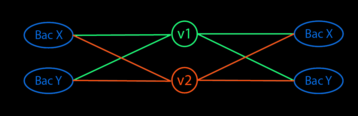
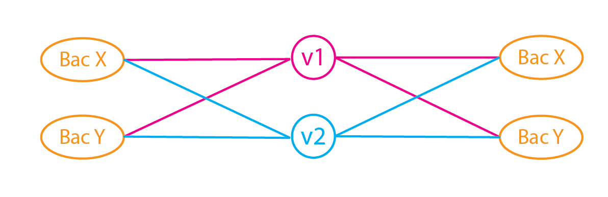
Another way to encode data is to use an autoencoder (AE). The autoencoder first encodes data into a latent space (often of a smaller dimension than the input data) using one or more layers, and decodes points in the latent space back to the original data. The goal is learn features that reduce the difference between the original and reconstructed data.

Autoencoders are often compared to PCA. In fact, an autoencoder that is a single layer deep (1 for encoding, 1 for decoding) and uses linear activation is often thought to function like PCA in the roughest of sense. However, there are several differences between both methods.

PCA and covariance is primarily a linear operation. Their basic implementation cannot learn non-linear features the same way that autoencoders can. Kernel PCA is one way to extend linear PCA to non-linear data. PCA eigenvectors are orthorgonal by default whereas AE weights are not orthorgonal.

PCA transforms and reconstructs the data using the same transformation (eigenvector) matrix. The encoder and decoder layer on the other hand have different weights.

I will show that it is possible to configure an autoencoder to produce the same results as PCA and not just approximate it!

Note: Performing PCA using autoencoders makes little sense because the code is complicated and computationally intensive compared to PCA. However, if we can recreate PCA using an autoencoder, it means we can treat autoencoders as less of a ‘black box’ and more of a PCA analog which we can further improve on.

from numpy.random import seed
seed(123)

import sklearn
from sklearn import datasets
import numpy as np
from sklearn.model_selection import train_test_split
from sklearn.preprocessing import StandardScaler, MinMaxScaler
from sklearn import decomposition
import scipy

import tensorflow as tf
from tensorflow.keras.models import Model, load_model
from tensorflow.keras.layers import Input, Dense, Layer, InputSpec
from tensorflow.keras.callbacks import ModelCheckpoint, TensorBoard
from tensorflow.keras import regularizers, activations, initializers, constraints, Sequential
from tensorflow.keras import backend as K
from tensorflow.keras.constraints import UnitNorm, Constraint

Data

1. Generate data from cov matrix and mu
2. Preprocess data. Check out link

# Utility function
def correlation_from_covariance(covariance):
    v = np.sqrt(np.diag(covariance))
    outer_v = np.outer(v, v)
    correlation = covariance / outer_v
    correlation[covariance == 0] = 0
    return correlation

# Generate Data
n_dim = 5 # 5 dimensional data
cov = sklearn.datasets.make_spd_matrix(n_dim, random_state=1234) # Generate
corr = correlation_from_covariance(cov)
mu = np.random.normal(0, 0.1, n_dim) # Generate mean
n = 1000 # Number of samples
X = np.random.multivariate_normal(mu, cov, n)
#X = X.astype('float32')

# Preprocess data
X_train, X_test = train_test_split(X, test_size=0.01, random_state=123)
scaler = StandardScaler() #Translate data and scale them such that stddev is 1
scaler.fit(X_train)
X_train_scaled = scaler.transform(X_train)
X_test_scaled = scaler.transform(X_test)

PCA

We first perform a standard PCA. As a recap, PCA is simply the eigendecomposition the covariance matrix. To get a graphical intuition of what PCA does, we need to understand what the covariance matrix. Graphically, for 2D data, the covariance matrix describes the shape of the data on a plane. It is basically a transformation matrix that shapes data distributed in a circle (cov(x,y)=0, var(x)=1, var(y)=1) into a skewed ellipse.

When we perform eigendecomposition, we are essentially breaking down the transformation into separate scaling and skewing/rotating operations. The eigenvector matrix unskews the data, and a diagonal eigenvalue matrix scales the data. Note that the eigenvalues are the variance of the data along the eigenvectors i.e. the lengths of the major and minor axis of the ellipse.

We will perform PCA using

1. Original COV
2. Derived COV

To check if the vectors are in the same direction, we perform a dot product of the unit vectors. If the value is close to 1 i.e the eigenvectors from both COV matrix have very similar directions.

# Original COV
values, vectors = scipy.linalg.eig(corr) # Vector are columns
idx = np.argsort(values*-1)
values, vectors = values[idx], vectors[:,idx]
ratio = values/values.sum() # Explained Variance Ratio

# Derived COV
pca_analysis = sklearn.decomposition.PCA()
pca_analysis.fit(X_train_scaled)
cov2 = pca_analysis.get_covariance()
vectors2 = pca_analysis.components_ # Vector are rows
values2 = pca_analysis.explained_variance_
ratio2 = pca_analysis.explained_variance_ratio_
cov2, corr
# Compare eigenvectors and eigenvalues
values, values2
vectors.T, vectors2
cross_prod = []
for i in range(n_dim):
    cross_prod.append(np.dot(vectors.T[i], vectors2[i])/(scipy.linalg.norm(vectors.T[i])*scipy.linalg.norm(vectors2[i])))

print(cross_prod)

Autoencoder

I’ll first demonstrate how to create an autoencoder in tensorflow using the basic layers. Since I’ll need to customize the training loop later, it is easier to create a tensorflow model using subclass instead of sequential or functional API.

Set up model and layers

nb_epoch = 100 #Number of runs
batch_size = 16
input_dim = X_train_scaled.shape[1] #Number of predictor variables,
encoding_dim = 2
learning_rate = 1e-2

# Batch and shuffle data
train_ds = tf.data.Dataset.from_tensor_slices(
    (X_train_scaled, X_train_scaled)).shuffle(1000).batch(batch_size)

test_ds = tf.data.Dataset.from_tensor_slices((X_test_scaled, X_test_scaled)).batch(batch_size)

# Define model
class MyModel(Model):
    def __init__(self):
        super(MyModel, self).__init__()
        # Define the layers
        self.d1 = Dense(encoding_dim, activation="linear", input_shape=(input_dim,), use_bias=True, dtype='float32')
        self.d2 = Dense(input_dim, activation="linear", use_bias = True)

    def call(self, x):
        # Connecting the layers
        x = self.d1(x)
        return self.d2(x)

# Create an instance of the model
tf.keras.backend.clear_session()
model = MyModel()

Select Loss function, Optimzer and Metric

We define the loss function using mean squared error to evaluate the difference between the original and reconstructed data. The model optimize its weights using stochastic gradient descent, i.e. training the model using a gradients from a subset of input data. The loss metric is the mean of losses (MSE) for all data.

Note: For sequential models, when choosing a loss metric in the model.compile() step, you may see ‘accuracy’ chosen in some examples. They don’t make sense in a autoencoder since it is meant for categorial data, not continuous data.

autoencoder.compile(metrics=['accuracy'],
                    loss='mean_squared_error',
                    optimizer='sgd')

• Tensorflow Issue #34451 - if you pass the string ‘accuracy’, we infer between binary_accuracy/categorical_accuracy functions
• See more discussion here

loss_object = tf.keras.losses.MeanSquaredError()
optimizer = tf.keras.optimizers.SGD(learning_rate=learning_rate)

train_loss = tf.keras.metrics.Mean(name='train_loss')
test_loss = tf.keras.metrics.Mean(name='test_loss')

Set up training steps and train network

# Define training step
@tf.function
def train_step(input, output):
      with tf.GradientTape() as tape:
            predictions = model(input)
            loss = loss_object(output, predictions)
      # Backpropagation
      gradients = tape.gradient(loss, model.trainable_variables)
      optimizer.apply_gradients(zip(gradients, model.trainable_variables))
      # Log metric
      train_loss.update_state(loss)

@tf.function
def test_step(input, output):
    # training=False is only needed if there are layers with different
    # behavior during training versus inference (e.g. Dropout).
    predictions = model(input)
    t_loss = loss_object(output, predictions)
    # Log metric
    test_loss(t_loss)
    #test_accuracy(output, predictions)

    for epoch in range(nb_epoch):
        # Reset the metrics at the start of the next epoch
        train_loss.reset_states()
        test_loss.reset_states()

        for num, (input, output) in enumerate(train_ds):
            train_step(input, output)

        for input, output in test_ds:
            test_step(input, output)

        template = 'Epoch {}, Loss: {}, Test Loss: {}'
        if (epoch) % 10 ==0:
            print(template.format(epoch,
                            train_loss.result(),
                            test_loss.result()))

To be continued in Part 2.