Can a neural network perform PCA? Part 2 - The transformation

11 minute read

PCA-like Autoencoder

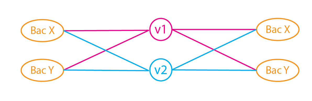
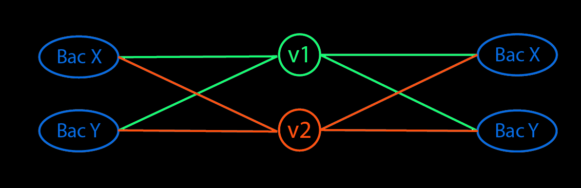
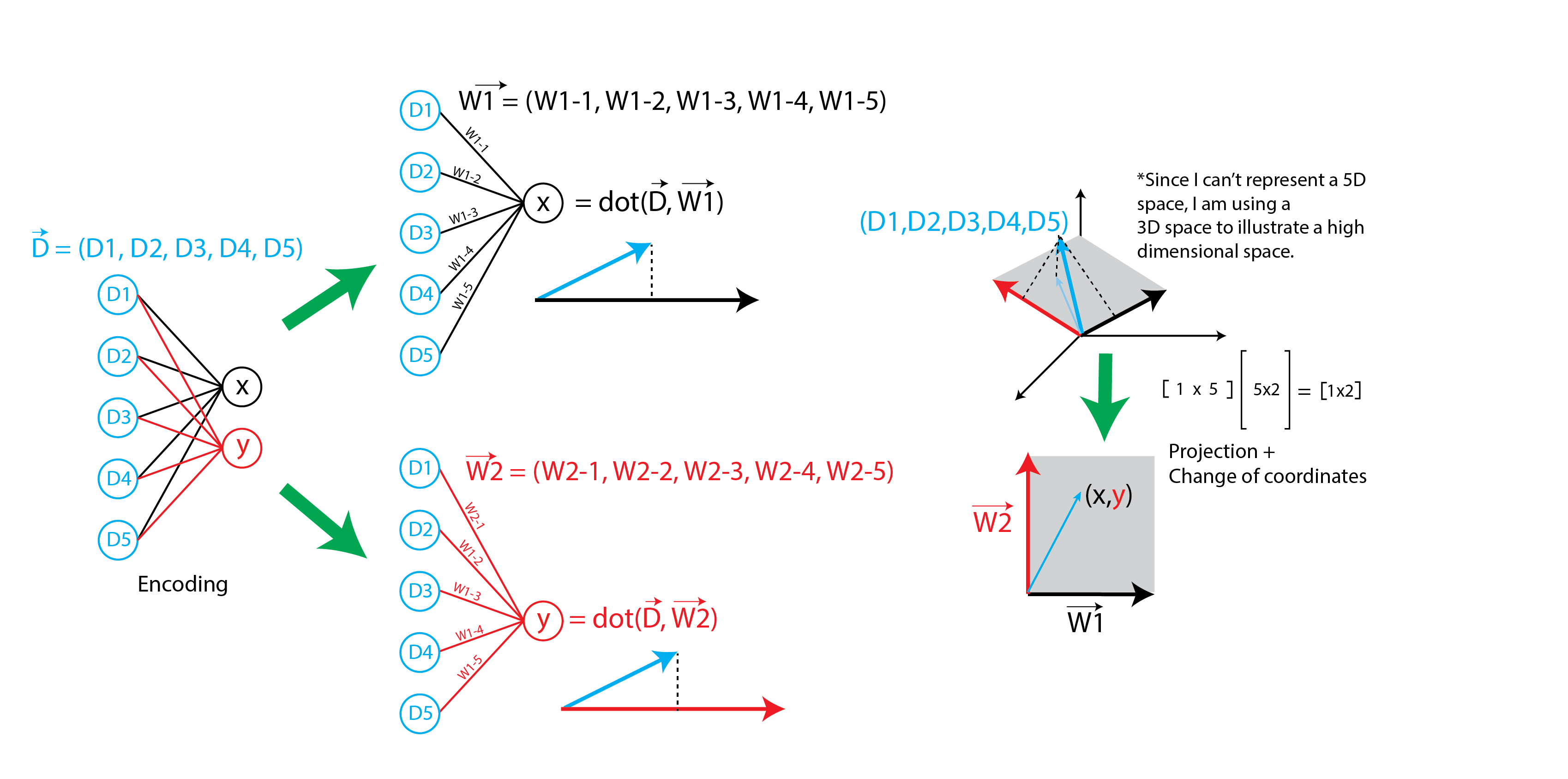
The goal of creating a PCA-like autoencoder is to provide context to the underlying weights of the neural network. In a neural network, for linear activation, the first layer is essentially a projection of the data onto a space determined by the weights of the layer. The cartoon below illustrates how a neural network projects data onto a vector space determined by the weights. To avoid confusion, all subsequent mentions of weights refer to the weight vectors as shown in the figure.

We will now introduce the following features to the autoencoder to replicate PCA:

encoder and decoder share the same weights but tranposed.*
1. tied weight do not extend to biases
linear activations.
orthogonal weights.
unit length weights
encoder dimension increased and trained iteratively. Weights of previously trained dimensions are kept constant. This replicates the process of finding the eigen vector that best explains the data iteratively.
loss function that minimizes variance of data in the latent space since we want the weights to function like eigenvectors.**

*Note that the decoder is not strictly the inverse of the encoder. However, in the case of a PCA, the transpose of the unit eigenvector matrix is also the inverse, so if we transpose the weights of the encoder, we get a decoder that is effectively performing an inverse operation. For encoders with smaller dimension, the inverse operation is technically a pseudoinverse.

** Turns out, we don’t need to create such a loss function explicitly since the autoencoder will try to minimize variance naturally for the MSE loss function. See discussion on AE at the end.

As we will show later, choosing either tied-weights, orthogonality weights or sequential training is sufficient for generating weights that are orthogonal, though only sequential training ensures that the weights are the same as PCA’s eigenvectors.

Adding orthogonality regularizer

To ensure that the weights are orthogonal, we add a regularizer that penalizes weights that are not orthogonal. A quick way to define one is to recognize that if A is an orthonormal matrix, transpose(A) = inverse(A). If we multiply the orthonormal weight matrix by their transpose, we should get an identity matrix. Any deviation means the weights are not orthonormal, and we penalize it by adding the difference to the loss function.

Note that we are not making this a constraint since we want the autoencoder to be able to choose slightly non-orthogonal weights if it results in a better fit, and an orthogonality regularizer is easier to implement.

See link for more details on the math.

class Orthogonal(tf.keras.regularizers.Regularizer):
    def __init__(self, encoding_dim, reg_weight = 1.0, axis = 0):
        self.encoding_dim = encoding_dim
        self.reg_weight = reg_weight
        self.axis = axis

    def __call__(self, w):
        if(self.axis==1):
            w = K.transpose(w)
        if(self.encoding_dim > 1):
            m = K.dot(K.transpose(w), w) - K.eye(self.encoding_dim)
            return self.reg_weight * K.sqrt(K.sum(K.square(K.abs(m))))
        else:
            m = K.sum(w ** 2) - 1.
            return m

Sequential training

A unique feature of the PCA is that each eigenvector accounts for some variance in the data in increasing order. However, in an autoencoder, the loss function is defined only by the accuracy of the reconstructed data. If we set the latent space to have the same dimension as the incoming data, it is possible for the autoencoder to find a set of orthogonal weights that transforms the data to a different latent space and back perfectly, but the weights are more a reflection of the initial condition than useful information.

If the dimension of the latent space is smaller than that of the input, the weights need to compress the data more efficiently (i.e. account for as much variance in the data as possible), which constraints the weights slightly. However, there are still many ways to ‘distribute’ the data variance across different weight vectors, so the values are again dependent on the initialization. Put another way, if the encoding layer is 2D, there is a plane that best describes the data variance. As I show later, the autoencoder is capable of finding the plane, but may represent the plane with two different vectors compared to PCA.

If we reduce the encoding layer to a dimension of 1, the one resulting weight vector has to account for as much variance as possible. Naturally, it has to be close to the first principle component (due to the tied weights regularization) and the variance of the projected data must be close to the first eigenvalue.

Once we have found the first weight vector, we can fix it while training the second weight vector, subject to the same constraints as before. The autoencoder should in theory find a second weight vector that accounts for the second most variance of the data. We repeat this for all subsequent weights until the desired encoding dimension is achieved.

Below, we introduce a new layer that generates seperate weight vectors instead of a kernel matrix. By declaring the weight vectors separately, we can train them individually while keeping previously trained vectors fixed. Additionally, all untrained weights should be set to zero so that they don’t affect the training. When a weight vector is ready to be trained, change it from zero to the default kernel_initializer so that the model can learn more efficiently. weight_ind is defined as the index of the weight that is currently being trained. When calling the layer, the layer uses weight_ind to generate the appropriate kernel for training.

from tensorflow.python.ops import math_ops, sparse_ops, gen_math_ops, nn
from tensorflow.python.framework import tensor_shape

class DenseWeight(tf.keras.layers.Dense):
    # source code for tf.keras.layers.Dense -> https://bit.ly/3ciTIEJ
    def __init__(self, units, w_axis, **kwargs):
        # w_axis (0 or 1) determines which axis the weight vectors are on.
        # For encoder -> w_axis = 0, decoder -> w_axis = 1
        super(DenseWeight, self).__init__(units, **kwargs)
        self.w_axis = w_axis

    def build(self, input_shape):
        super(DenseWeight,self).build(input_shape)
        last_dim = tensor_shape.dimension_value(input_shape[-1])
        self.kernelshape = [last_dim, self.units]
        self.weightshape = [1,1]
        self.weightshape[self.w_axis] = self.kernelshape[self.w_axis]
        self.kernelall = []
        # Setting separate weight vectors.
        for i in range(self.kernelshape[int(not self.w_axis)]):
            custominit = self.kernel_initializer
            self.kernelall.append(self.add_weight(
            name='w{:d}'.format(i), shape=self.weightshape,
            initializer=custominit, regularizer=self.kernel_regularizer,
            constraint=self.kernel_constraint, dtype=self.dtype,
            trainable=True))

    def call(self, inputs, weight_ind=None):
        # Set default
        if weight_ind is None:
            weight_ind = len(self.kernelall)-1
        # Create kernel where the weights above weight_ind are zero so that they don't affect the training.
        self.kerneltrain = [w if w_ind <= weight_ind else tf.zeros(w.shape) for w_ind, w in enumerate(self.kernelall)]
        self.kernel = tf.concat(self.kerneltrain,int(not self.w_axis))
        # Copied from source
        return super(DenseWeight,self).call(inputs)

Performing sequential training

To specify which vector to train, we define var_list, which is used by the optimizer to determine which variable to train. Note that var_list should not be defined in train_step since it uses python features that are not compatible with @tf.function. See link.

# Create an instance of the model
tf.keras.backend.clear_session()
model = TiedModel()

# Select Loss function, Optimizer and Metric
loss_object = tf.keras.losses.MeanSquaredError()
optimizer = tf.keras.optimizers.SGD(learning_rate=learning_rate)

train_loss = tf.keras.metrics.Mean(name='train_loss')
test_loss = tf.keras.metrics.Mean(name='test_loss')

# Define training step
@tf.function
def train_step(input, output, d1_weight_ind, var_list):
      with tf.GradientTape() as tape:
        predictions = model(input, d1_weight_ind)
        loss = loss_object(output, predictions)
      # Backpropagation
      gradients = tape.gradient(loss, var_list)
      optimizer.apply_gradients(zip(gradients, var_list))
      # Log metric
      train_loss.update_state(loss)


@tf.function
def test_step(input, output):
    # training=False is only needed if there are layers with different
    # behavior during training versus inference (e.g. Dropout).
    predictions = model(input)
    t_loss = loss_object(output, predictions)
    # Log metric
    test_loss(t_loss)
    #test_accuracy(output, predictions)


nb_epoch = 31 #number of epochs per weight vector
d1_weight_ind = 0
while d1_weight_ind <= encoding_dim-1:
    for epoch in range(nb_epoch):
        # Reset the metrics at the start of the next epoch
        train_loss.reset_states()
        test_loss.reset_states()

        for num, (input, output) in enumerate(train_ds):
            var_list = []
            untrainable_weights = [i for ind, i in enumerate(model.d1.weights) if ind != d1_weight_ind]
            for v in model.trainable_variables:
                append = True
                for w in untrainable_weights:
                    if v is w:
                        append = False
                        break
                if append:
                    var_list.append(v)
            train_step(input, output, d1_weight_ind, var_list)

        for input, output in test_ds:
            test_step(input, output)

        template = 'Epoch {}, Loss: {}, Test Loss: {}'
        if epoch % 10 == 0:
            print(template.format(epoch,
                            train_loss.result(),
                            test_loss.result()))

    d1_weight_ind+=1

Comparing weights

Let’s compare weights/eigenvectors and projected data variance/eigenvalues.

Orthorgonality

The dot product of the eigenvector matrix enc_weights and its transpose is approximately the identity matrix i.e. the weights are orthogonal.

Eigenvalues and Eigenvectors

The ‘eigenvalue’ of the a weight vector can be obtained by projecting the data onto the vector and calculating the resulting variance. We shall call the variance the projected variance.

The eigenvalues and eigenvectors for very close to the weights and projected variance.

Eigenvector directions

We can further test the direction of the eigenvector vs weights by taking the dot product of their unit vectors. The closer they are to 1, the smaller the angle between the vectors.

enc_weights = tf.concat(model.d1.weights,axis=1).numpy()
print('Check Orthogonality\n{}\n'.format(np.dot(enc_weights.T,enc_weights))) # Check for weight orthogonality
enc_values = np.dot(X_train_scaled, enc_weights).var(axis=0) # Get variance / eigenvalue
idx = np.argsort(enc_values*-1) # Sort the weights by data variance
values3, vectors3 = enc_values[idx], enc_weights[:,idx]

# Compare eigenvectors and eigenvalues
print('Original EigVal\n{}\nDerived EigVal\n{}\nAutoencoder DataVar\n{}\n'.format(values, values2, values3))
print('Original PC\n{}\nDerived PC\n{}\nAutoencoder Weights\n{}\n'.format(vectors.T, vectors2, vectors3.T))

# Compare direction of PCA eigenvectors and AE weights
def dp(a,b):
    #pseudo
    return np.dot(a, b)/(scipy.linalg.norm(a)*scipy.linalg.norm(b))

dot_prod = []
for i in range(vectors3.T.shape[0]):
    dot_prod.append(dp(vectors2[i], vectors3.T[i]))

print('Dot product of PCA eigenvectors and AE weights')
print(dot_prod)

Comparing loss between original autoencoder and PCA-like autoencoder

Comparing the loss, it looks like the autoencoder performs similarly regardless of the PCA-inspired modifications. It suggests that the linear autoencoder is capable of finding the same latent space that best represents the data (i.e. the latent space that best reduces MSE) regardless of modifications. The reason the weights are different is because the autoencoder choose to represent the same latent space using different weight vectors depending on the initialization. By applying sequential training, the autoencoder selects meaningful vectors that are sorted by their power to reduce data variance. In fact, in PCA_seqtrainonly.py, sequential training alone of both encoder and decoder (i.e. training the first weight vector of encoder and decoder together followed by the second weight vector and so on) is sufficient for generating orthogonal weights, making the other modifications redundant!

Another interesting feature is the redundancy of tied-weights and orthogonality regularization. Let’s suppose for now that the unconstrained autoencoder returns orthogonal weights. If data dimension and encoding dimension are equal, the decoder simply takes the transpose (inverse) of the encoder weights to reconstruct the data perfectly. If encoding dimension is smaller, the transpose won’t give us a perfect reconstruction, but one that minimizes MSE. The transpose of a non-square orthogonal matrix is also known as the pseudoinverse matrix. Conversely, if we tie the weights between encoder and decoder (via a transpose), the learned weights must be orthogonal since the loss is the same either way. Note that the redundancy only holds if the loss criteria is MSE. See PCA_tiedonly.py for more details.

TL;DR Either one of these modifications, sequential training; tied-weights or orthogonality regularization, guarantees orthogonal weights when coupled with MSE loss. Only sequential training sorts the weights by ‘eigenvalues’ and matches the eigenvectors from PCA.

Configuring the latent space

Since the AE learns the same latent space except with different representation, we can learn the PCA representation by applying PCA to the latent space. The new eigenvectors will be in terms of the latent space representation, so to get back the depedence on the original input variables, apply a pseudo inverse.

Pseudoinverse matrix and autoencoder

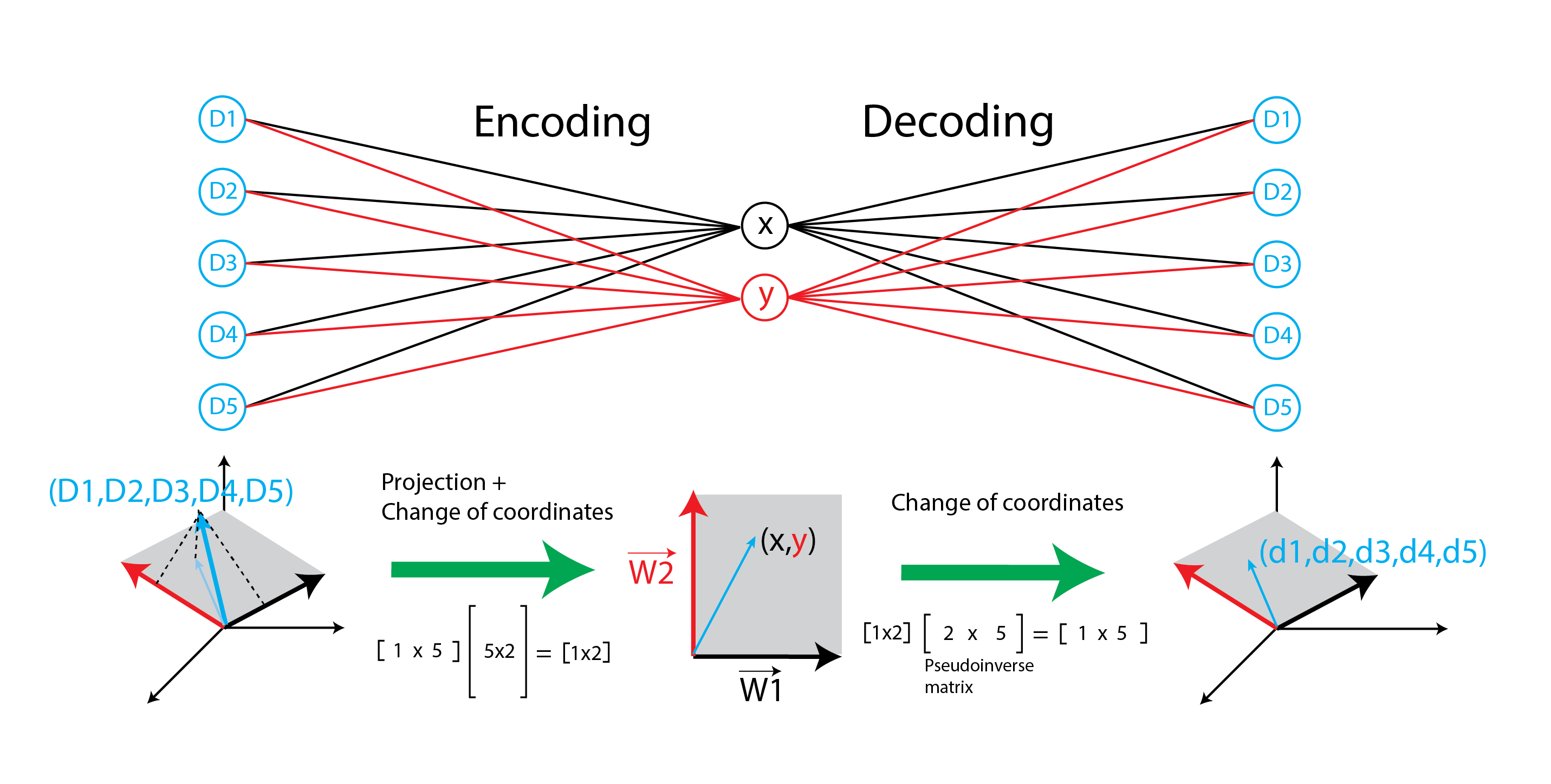
Now let’s suppose that the unconstrained autoencoder returns weights that are non-orthogonal. Since the autoencoder is representing the same optimal latent space with non-orthogonal weights, simply taking a transpose to decode the data will not work. Nevertheless, the decoder is able to find a set of weights that minimizes MSE. Turns out, the decoder weights match the pseudoinverse matrix calculated using SVD or np.linalg.pinv. The encoder projects data onto a latent space and transforms its coordinates, the decoder merely transforms the coordinates back but without ‘unprojecting’ the data, as shown in the cartoon below. An interesting property of pseudoinverse matrices is that multiplying a matrix by its pseudoinverse will yield an identity matrix (in the smaller dimension). See link for more details on pseudoinverse matrices.

Conclusion

A linear autoencoder with MSE loss performs similarly to PCA. Given enough epochs, it’ll find the same latent space as as the one found by PCA to minimize variance. The modifications proposed here do affect the latent space. Instead, they help the autoencoder look for vector representation of the latent space that are both interpretable and meaningful.

Futher insights and future work

Given that MSE loss function is key to finding the right latent space that minimizes variance, using a different the loss function will produce a latent space that optimizes other characteristic in the data.
Biases matter if the data was not preprocessed. However, it complicates PCA <-> autoencoder analogy since biases don’t have a simple inverse operation the same way weight matrices can be transposed.
Non-linearity can be achieved by using non-linear activation, or by changing the number of layers?
The first layer projects the data onto an optimal latent space and determines the bulk of the compression. i.e. if the first encoding dimension is small, the subsequent layers won’t be able to recover information that’s lost.
The second/subsequent layers would look for trends in the latent space and alter it, such as prioritizing locality in the latent space for data sharing the same label. (See VAE)
Fourier compression essentially transforms signals to frequency components and removes high frequency ones. Analagously, autoencoder transforms data to a different latent space and projects them onto important vectors in a single step.

Twitter Facebook LinkedIn

Jonathan Teo